Simulating SMART designs with sim_treatment

Building two-stage SMARTs step by step

Introduction

The sim_treatment() function provides a flexible way to simulate treatment assignments one stage at a time. It can be used to simulate various common SMART designs, including those with response indicators or feasible sets. An additional function block_rand() can implement permuted block randomization to ensure greater balance than binomial randomization in later stages.

This vignette walks through three two-stage designs:

1. No response status — all participants are re-randomized at stage 2.
2. Response, non-responders only — a response indicator is observed between stages and only non-responders are re-randomized.
3. Response, everyone re-randomized — a response indicator is observed but both responders and non-responders receive a new randomization at stage 2.

The first stage helps to build our intuition in the simplest case. The second and third showcase additional features of the function. Each section includes a diagram of the design, sample simulation code, and the resulting data.

library(rsmart)

Design 1: No response status

In the simplest two-stage SMART, every participant is randomized at stage 1 and again at stage 2 regardless of any intermediate outcome. This design has four embedded treatment regimes.

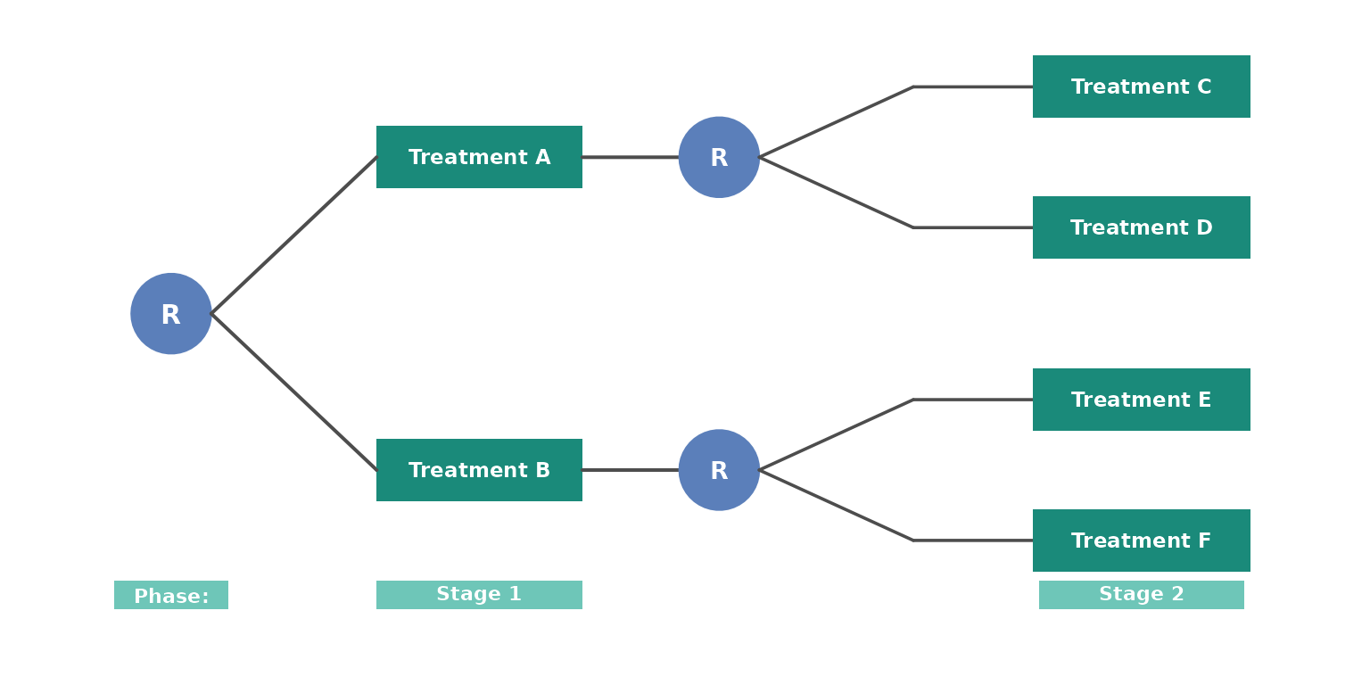
Design 1: Two-stage SMART without a response. All participants are re-randomized at stage 2.

This design has four embedded regimes: (A, C), (A, D), (B, E), and (B, F), which will be encoded as (a1=0, a2=0), (a1=0, a2=1), (a1=1, a2=0), (a1=1, a2=1), respectively, using sim_treatment().

Simulation

Consider a possible trial with 500 participants. The age of participants is recorded at entry and their compliance with treatment at stage 2. We assign treatments with equal randomization using a permuted block design.

We provide sim_treatment() with:

• n_treatments: the number of treatments available at the stage for randomized participants
• dat: a dataset with the initial covariates and IDs at the first stage
• stage: the stage of the trial that treatments should be assigned for
• rand_prob_fn: the block_rand function to generate permuted block randomization, with each treatment repeated twice in a block

The block_rand function here will use a block size of 4 so a sample block could be 2 1 1 2. This will ensure that treatment imbalance between groups is minimized.

Because there is no response status, the input randomize_response is implicitly left at its default (NULL).

The function will return the data frame with the treatment assignment for each participant.

set.seed(42)
n <- 500

# Start with baseline data
dat1 <- data.frame(
  id  = 1:n,
  x1  = round(runif(n, 25, 75)),        # age
  x2  = rbinom(n, 1, 0.9)               # treatment compliance
)

# Stage 1: block randomization
dat1 <- sim_treatment(n_treatments = 2, dat = dat1, stage = 1,
                      rand_prob_fn = block_rand(block_rep = 2))

# Stage 2: everyone is re-randomized within a1 groups (no response)
dat1 <- sim_treatment(n_treatments = 2, dat = dat1, stage = 2,
                      rand_prob_fn = block_rand(block_rep = 2))

table(dat1$a1, dat1$a2)
#>    
#>       0   1
#>   0 124 126
#>   1 125 125
head(dat1)
#>   id x1 x2 a1 a2
#> 1  1 71  1  1  0
#> 2  2 72  1  0  1
#> 3  3 39  1  1  1
#> 4  4 67  1  0  1
#> 5  5 57  1  1  0
#> 6  6 51  1  0  0

We see that the resulting data set has the columns id, x1, x2, a1, a2. The treatments are appended as a<stage>.

Design 2: Only non-responders are re-randomized

Commonly, tailoring variables are used in SMARTs to determine sequential treatment options. A response indicator is observed between stages and then governs available treatements. Often, it may be unethical to re-randomized away from a treatment that is working well and responders are given a second stage treatment deterministically. Alternatively, non-responders may be discontinued or given a single salvage therapy. Here we encode this status using r2 and will assign responders r2 = 1 a single treatment (coded a2 = 0). Non-responders will be re-randomized.

In the case where responders are randomized and non-responders are not, then the encoding of r2 = 1 represents non-responders and the function sim_treatment will assign responders, now encoded as r2 = 0, treatments.

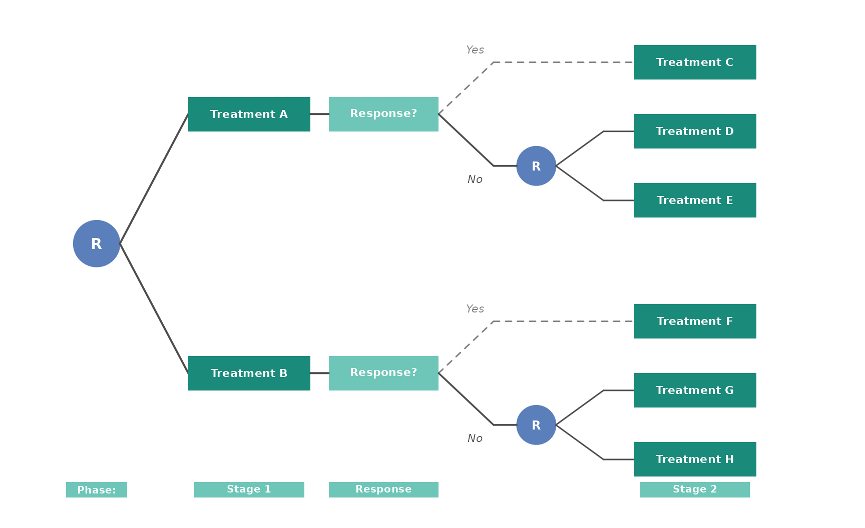
Design 2: Two-stage SMART where only non-responders are re-randomized at stage 2.

Responders follow a deterministic path (dashed lines). There are still four embedded regimes, but now follow rules “give treamtent 1 at stage 1, if response give treatment 2 at stage 2, otherwise give treatment 3 at stage 2. (1, 2, 3)” The embedded regimes are now encoded as: (a1=0, a2=0, a2=0), (a1=0, a2=0, a2=1), (a1=1, a2=0, a2=0), (a1=1, a2=0, a2=1).

Simulation

We use similar inputs as before, but with the additional input randomize_response = "N" so that we assign a2 = 0 to all responders and randomize only the non-responders within each a1 group.

set.seed(42)
n <- 500

dat2 <- data.frame(
  id  = 1:n,
  t1  = sort(round(runif(n, 0, 365 * 2))),  # enrollment day
  x1  = round(runif(n, 25, 75))             # age
)

# Stage 1: block randomization (data sorted by t1)
dat2 <- sim_treatment(n_treatments = 2, dat = dat2, stage = 1,
                      rand_prob_fn = block_rand(block_rep = 2))

# Generate response and stage 2 timing
dat2$r2 <- rbinom(n, 1, 0.5)
dat2$t2 <- dat2$t1 + 100 + round(runif(n, -10, 10))

# Sort by t2 before stage 2 randomization (see note below)
dat2 <- dat2[order(dat2$t2), ]

# Stage 2: only non-responders re-randomized
dat2 <- sim_treatment(n_treatments = 2, dat = dat2, stage = 2,
                      rand_prob_fn = block_rand(block_rep = 2),
                      randomize_response = "N")

table(dat2$a1, dat2$a2, dat2$r2,
      dnn = c("a1", "a2", "r2"))
#> , , r2 = 0
#> 
#>    a2
#> a1    0   1
#>   0  58  58
#>   1  62  63
#> 
#> , , r2 = 1
#> 
#>    a2
#> a1    0   1
#>   0 134   0
#>   1 125   0

Because of the use of the permuted block randomization, we see that among responders and conditioned on the first treatment, there is relative balance between treatment assignments. All responders r2 = 1 received a2 = 0.

Design 3: Both responders and non-responders re-randomized

In some SMARTs, all participants are re-randomized at stage 2, with treatments allowed to vary by response status. This means responders may or may not receive different second-stage treatments than non-responders, and the randomization probabilities or allocation schedules can differ between the two groups.

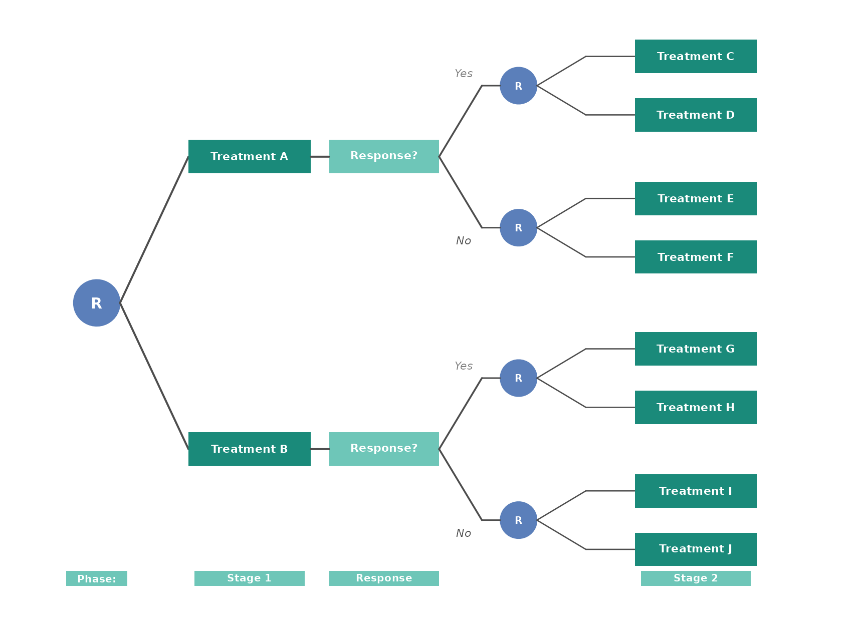
Design 3: Two-stage SMART where both responders and non-responders are re-randomized at stage 2.

Because both responders and non-responders are randomized at stage 2, the number of embedded regimes grows. With the canonical encoding, each regime specifies a stage-1 treatment, a responder stage-2 treatment, and a non-responder stage-2 treatment, yielding \(2 \times 2 \times 2 = 8\) embedded regimes. For completeness, we can enumerate these regimes as follows:

1. (0, 0, 0)
2. (0, 0, 1)
3. (0, 1, 0)
4. (0, 1, 1)
5. (1, 0, 0)
6. (1, 0, 1)
7. (1, 1, 0)
8. (1, 1, 1)

Again, using the same format where these are the treatments given at stage 1, at stage 2 for responders, and at stage 2 for non-responders.

Simulation

Setting randomize_response = "Y" includes the response column r2 in the grouping variables so that randomization is performed independently within each combination of a1 and r2.

set.seed(42)
n <- 500

dat3 <- data.frame(
  id  = 1:n,
  t1  = sort(round(runif(n, 0, 365 * 2))),
  x1  = round(runif(n, 25, 75))
)

# Stage 1
dat3 <- sim_treatment(n_treatments = 2, dat = dat3, stage = 1,
                      rand_prob_fn = block_rand(block_rep = 2))

# Generate response and timing
dat3$r2 <- rbinom(n, 1, 0.5)
dat3$t2 <- dat3$t1 + 100 + round(runif(n, -10, 10))

# Sort by t2 before stage 2
dat3 <- dat3[order(dat3$t2), ]

# Stage 2: responders AND non-responders randomized (stratified by response)
dat3 <- sim_treatment(n_treatments = 2, dat = dat3, stage = 2,
                      rand_prob_fn = block_rand(block_rep = 2),
                      randomize_response = "Y")

table(dat3$a1, dat3$a2, dat3$r2,
      dnn = c("a1", "a2", "r2"))
#> , , r2 = 0
#> 
#>    a2
#> a1   0  1
#>   0 58 58
#>   1 62 63
#> 
#> , , r2 = 1
#> 
#>    a2
#> a1   0  1
#>   0 67 67
#>   1 62 63

Unlike Design 2, responders now receive both a2 = 0 and a2 = 1. We again see that conditioned on response status and first treatment, the a2 assignments are relatively well-balanced.

Note on ordering and block randomization

When using block_rand() (or any allocation-schedule–based randomization), the order in which participants appear in the data frame determines their position in the allocation schedule. If enrollment timing matters — for example, in a group sequential design — the data should be sorted by the relevant time variable before calling sim_treatment() at each stage.

For stage 1, sort by the enrollment time (e.g., t1):

dat <- dat[order(dat$t1), ]
dat <- sim_treatment(n_treatments = 2, dat = dat, stage = 1,
                     rand_prob_fn = block_rand(block_rep = 2))

For stage 2 and beyond, sort by the time of re-randomization (e.g., t2):

dat <- dat[order(dat$t2), ]
dat <- sim_treatment(n_treatments = 2, dat = dat, stage = 2,
                     rand_prob_fn = block_rand(block_rep = 2),
                     randomize_response = "N")

This ensures that the permuted block allocation schedule aligns with the temporal order of participant arrivals at each decision point. If simple randomization (the default rand_prob_fn) is used instead of block randomization, the row order does not affect the allocation and sorting is not required.