Algorithmic Process Optimization (APO) Workflow#
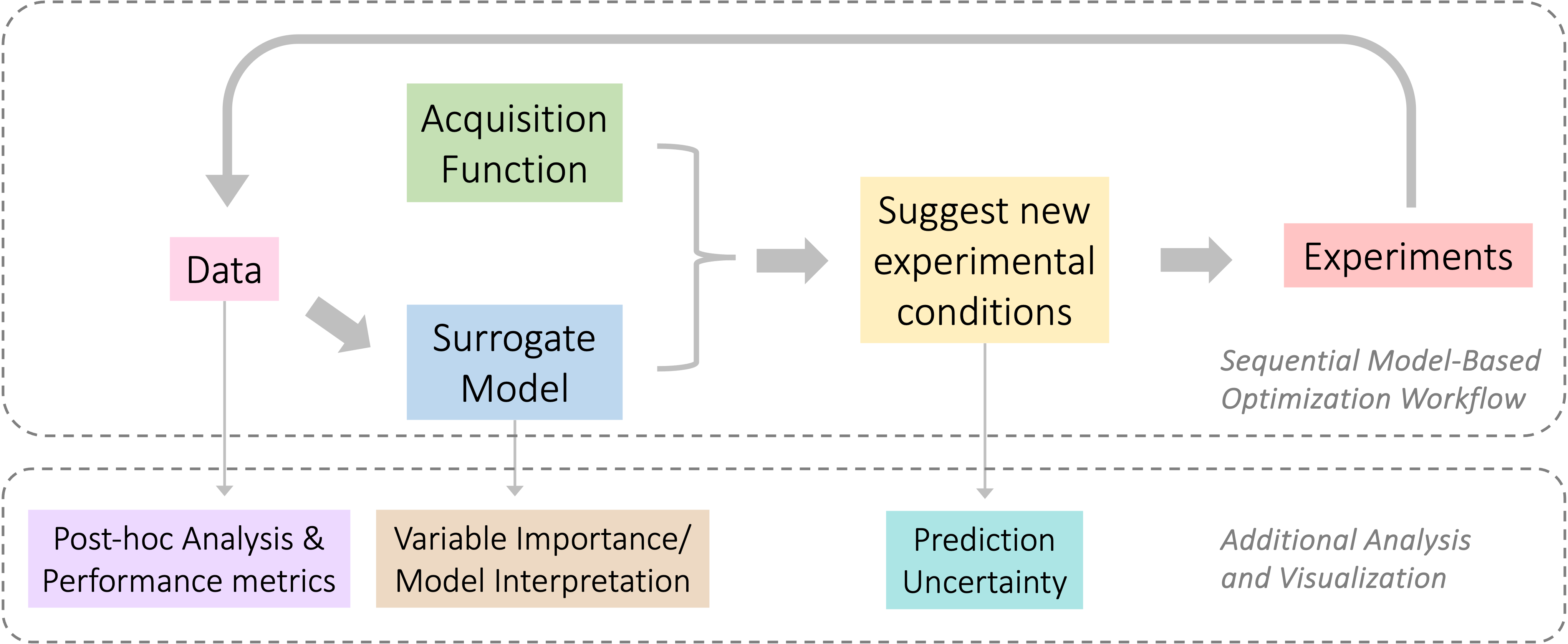
APO is an iterative procedure used for optimizing complex systems with an expensive-to-evaluate objective function. The major steps involve constructing a surrogate model to approximate the objective function and defining an acquisition function based on user preference that explores and/or exploits the design space to find the optimal solution.
When applied to chemical process optimization, the APO algorithms can effectively identify desirable experimental conditions or parameter settings that maximize process efficiency, minimize costs, or achieve other specified objectives within given resource constraints.
The components typically involved in APO algorithms are illustrated in the figure below:
In this obsidian library:
The Optimizer class object in optimizer submodule is the main portal that connects all the key components in the APO algorithm.
The dash submodule contains the source code for a web GUI using the Dash library.
The demo folder contains step-by-step Jupyter notebook usage examples as well as scripts for benchmark studies.
Data#
The data structure in a typical APO work flow includes:
\(X\): Experimental conditions, also called input features/parameters or independent variables. Usually a set of <20 variables are chosen to investigate their effects on the experimental outcomes. Various types of variables are supported:
Continuous variables:
Continuous (numerical) variable: A variable that can have an infinite number of real values within a given interval (e.g. Temperature)
Observational (numerical) variable: A variable that can be measured but not directly controlled, which still is useful for model fitting and optimization (e.g. Reaction time)
Discrete variables:
Discrete (numerical) variable: A variable that have finite number of numerical values within a given range or list of numbers (e.g. Buffer pKa)
Ordinal variable: A discrete variable that is defined by a meaningful ordered relationship between different categories (e.g. Light intensity at Low, Medium, High)
Categorical variable: A discrete variable that describes a name, label, or category without a natural order (e.g. Catalyst name)
Task variable: A special categorical variable which requires that a distinct response be predicted for each task (e.g. Reactor type)
\(X_{space}\): Experimental design space, or input parameter constraints. The multidimensional parameter space within which the experimental conditions \(X\) could be chosen and manipulated.
For each continuous variable in \(X\), the range of min and max range should be specified.
For each discrete variable, the set of possible distinct values (categories) should be provided.
Before fitting, all variables in \(X_{space}\) are transformed to an encoded, unit-cube space that is amenable to machine-learning, especially for Gaussian Processes. Each variable type has a pre-defined encoder (e.g. min-max scaling for continuous, one-hot encoding for categorical). Optimization and prediction occurs in the encoded (transformed) spsace \(X_t\), but de-transformation is always applied at key steps to ensure user-interaction and analysis within the measured parameter space \(X\)
\(Y\): Experimental outcomes, also called responses or dependent variables. It is the measured response of a response and the target variable to be optimized when no objective function is defined. Depends on the number of outcomes chosen for optimization, \(Y\) could be either a scalar (single-objective optimization) or a vector (multi-objective optimization). For a multi-objective optimization problem, the user can specify whether to maximize or minimize each each element in the \(Y\) vector. The responses \(Y\) are usually scaled to zero-mean and unit variance \(f(Y)\) with or without additional transformation before fitting.
\(O(Y, X)\) Objectives, or objective functions. The target value which is sought to be maximized or minimized in an optimization campaign. Objectives can be defined to convert single-output experiments to multi-output optimizations (e.g. using penalized features), and multi-output experiments can be condensed to signle-output optimizations (e.g. using scalarization or weighting).
See section
Data
and submodule
parameters,
and submodule
objectives
for more details.
Surrogate Model#
Assume the true relationship between the experiment outcome and input is \(f(X)\), which is unknown since the random and/or systematic errors \(\epsilon\) always present in experiments.
The measured outcome could be denoted as \(Y(X) = f(X) + \epsilon\). When the variance of \(\epsilon\) is constant, the noise is homoscedastic; otherwise when the noise is heteroscedastic, where the variance of \(\epsilon\) could depend on \(X\), making the optimization problem more challenging.
The surrogate model \(\hat{f}(X)\) is a predictive model that approximate the underlying unknown relationship \(f(X)\). The \(\hat{f}(X)\) has the same dimension as \(Y\). If \(Y\) is a vector, the experimental outcomes could be modeled jointly with multivariate multiple regression modeling methods at once; or each outcome could be modeled separately in parallel.
For Bayesian Optimization, surrogate models should provide both a point prediction (e.g. conditional mean given \(X\)) as well as a prediction uncertainty metric (e.g. conditional standard deviation given \(X\)). Most acquisition functions require both point prediction and uncertainty to balance the exploration and exploitation of the design space.
The most popular choice of surrogate model is Gaussian Process (GP) regression, which is a Bayesian model that combines prior knowledge with observed data to make probabilistic inferences of the posterior distribution. Under the assumption of Gaussian noise \(\epsilon\), it is cheap to compute the posterior mean and standard deviation for each new input data. Importantly, GP models do not provide a closed-form expression of \(f(X)\) but rather extimate a kernel which describes the covariance between unsampled \(X^*\) and sampled \(X\) space. Notably suitable for Bayesian Optimization, these kernels typically provide an increasing estimate of uncertainty as the distance from sampled space increases.
The APO workflow starts with collecting a set of initial experimental data \((X_0,Y_0)\), where the \(X_0\) could be random sampled from \(X_{space}\) or suggested by design-of-experiments methods. The initial surrogate model \(\hat{f}_0\) is then fit based on this initial dataset. At the \(i^{th}\) iteration later, an updated surrogate model \(\hat{f}_i\) is trained on all the available data \(\{X_t,Y_t\}_{1 \leq t \leq i}\). As more data are accumulated with multiple rounds of optimization, we expect the surrogate function to become more precise and better approximate the actual underlying functional relationship.
See section
Surrogate Model
and submodule
surrogates
for more details.
Acquisition Function#
The acquisition function aims to guide the search of promising new experimental conditions with the potential to achieve improved objectives. It usually depends on the surrogate model predictions and/or measured data , which scores any point in the \(X_{space}\).
In the \(i^{th}\) iteration, the acquisition function is
Maximizing this scoring function over the design space is used to produce the suggested new candidate conditions for the \((i+1)^{th}\) iteration:
The definition of acquisition function determines the trade-off between exploration and exploitation based on user preference.
Exploitation means leveraging existing knowledge by selecting new conditions that lead to optimal outcomes based on surrogate model prediction. It could maximize the immediate gains when the true relationship is relatively well understood and approximated by the surrogate model.
Exploration involves acquiring new information by sampling from less explored regions of the design space where the prediction uncertainty is higher. It may help to better understand the problem and improve surrogate model quality, which usually leads to better long-term outcomes or reveal new possibilities in the context of global optimization.
See section Acquisition Function,
submodule acquisition,
and submodule objectives
for more details.
Suggest New Experimental Conditions#
One or more new candidate experimental condition(s) are suggested based on the criteria of maximizing the acquisition function within the experimental design space. This can be done with individual sequential experiments m_batch=1 or parallized experiments m_batch>1 which can be optimized jointly optim_sequential=False or sequentially using fantasy models optim_sequential=True. More advanced constraints on input or output space that involves the combination or relationship of multiple input variables could be applied during the search.
With an accurate surrogate model and a well-designed acquisition function, the candidate point(s) which maximize the acquisition function are most likely to achieve improved experimental outcomes.
The optimization of acquisition function can be performed by analytical or numerical Monte-Carlo methods, depending on the complexity of acquisition functional form. The obsidian library relies heavily on the BoTorch library for MC-based Bayesian Optimization.
Please refer to section Tutorials for simulation studies that demonstrate the entire APO workflow as well as various visualization and analysis methods.